Hyperspectral Remote Sensing of Habitat Heterogeneity Between Tide-Restricted and Tide-Open Areas in the New Jersey Meadowlands
by Francisco J. Artigas¹ and Jiansheng Yang²
¹Meadowlands Environmental Research Institute, 1 DeKorte Park Plaza, Lyndhurst, NJ 07071
²Center for Information Management, Integration and Connectivity, Rutgers University, 180 University Ave., Ackerson Hall, Room 200, Newark, NJ 07102
Abstract
The restriction of tidal flow by roads, rail beds, dikes, and tide gates can significantly alter the integrity, spatial configuration, and ultimately the biodiversity of salt marshes. In our study we evaluated the effects of tide restriction on marsh habitat heterogeneity using hyperspectral remote sensing. Field-collected reflectance spectra of marsh surfaces and advanced image-classification techniques were applied to derive a thematic map of marsh surface types in the New Jersey Meadowlands from hyperspectral images captured by an airborne imaging spectroradiometer (AISA). Forty sampling sites were randomly selected in tide-restricted and tide-open areas and used to identify several landscape metrics for spatial pattern analysis. The results of this analysis showed significant differences in landscape metrics between tide-restricted and tide-open sites; open sites had a greater number, and a more even distribution, of landscape patch types. We found that the number of patches and the total edge were the best metrics for differentiating between tide-restricted and tide-open areas, and these may be used as surrogates for salt marsh biodiversity. The study indicated that hyperspectral images might be used on their own to detect marsh features that are ecologically significant.
Key words: hyperspectral remote sensing; landscape metrics; marsh; New Jersey Meadowlands; reflectance spectra; urban wetlands
Introduction
Tidal cycles of inundation and drainage are essential to the vitality of salt marshes as habitats for animal and plant species (Teal & Teal, 1969). The hydrological changes caused by restricting the flow of the tide with roads, rail beds, dikes, and tide gates significantly alter the integrity and spatial configuration of salt marshes in the northeastern United States. Visual interpretation of aerial photographs of marsh surfaces reveals an apparent decrease in marsh surface heterogeneity in tide-restricted regions (Thiesing, 2002). Coastal wetland restoration often involves reopening areas to the tide and creating new, more heterogeneous habitat to attract wildlife. Restoring surface habitat heterogeneity has been linked to an increase in the diversity of marsh species. For example, observations of bird-community composition in pre- and post-marsh-restoration projects have indicated that increased habitat heterogeneity after restoration significantly increased bird species richness (Delphey & Dinsmore, 1993; Brawley, Warren & Askins, 1998; Ratti, Rocklage, Giudice, Garton & Golner, 2001; Fletcher & Koford, 2003).
It is difficult to distinguish between various kinds of marsh surface types using traditional remote sensing technologies like aerial photography interpretation. Moderate-resolution remote sensors mounted on orbiting satellites (e.g., Landsat, with 30-meter* spatial resolution) are able to discriminate between surface types covering relatively large areas (Harvey & Hill, 2001; Berberoglu, Yilmaz & Ozkan, 2004), but they cannot reveal marsh features such as ponds, pannes, and levees whose extension is smaller than the image pixel size. Recently, imagery collected by hyperspectral sensors and near-infrared cameras and video technology mounted on low-altitude platforms (e.g., fixed-wing aircraft and balloons) has been widely applied in classifying wetland features in great detail (Miyamoto, Yoshino & Kushida, 2001; Shmidt & Skidmore, 2003). Using this new technology, it is possible to identify marsh surface types such as ponds. It is even possible to map plant species in coastal wetlands and relate their configuration and spatial arrangement to hydrological conditions influencing habitat heterogeneity—and ultimately, biodiversity.
We hypothesized that tide restriction causes the configuration and spatial arrangement of marsh surfaces to change, and that this rearrangement influences habitat heterogeneity. In order to characterize habitat heterogeneity based on the spectral reflectance of marsh surfaces, we identified a set of landscape metrics commonly used in the classification of hyperspectral imagery. These landscape metrics should illustrate that tide-restricted areas in marshlands have lower habitat heterogeneity than tide-open areas. Furthermore, we set out to show that it is possible to detect and identify tide-restricted and tide-open marshlands based only on landscape metrics derived from hyperspectral imagery. Demonstrating this could prove useful in the planning of coastal marsh preserves in fragmented urban wetlands, as discussed below.
The ramifications of scale are profound in studies in which habitat heterogeneity measurements are based on spatial metrics (Levin, 1992). Scale in our study had two components: the minimum mapping unit (2.5-meter pixel size) and the sample size (one-hectare—or 100-by-100-meter—plots). We selected 40 one-hectare sampling plots (20 in tide-restricted areas and 20 in tide-open areas) in the New Jersey Meadowlands from which to identify and calculate landscape metrics. We then compared the differences of these metrics between the tide-restricted and tide-open sites and evaluated the effects of tide restriction on habitat heterogeneity using spatial pattern analysis.
Methods
Study Area
Our study focused on the remaining marshlands of the New Jersey Meadowlands in northern New Jersey. Originally, the Meadowlands consisted of approximately 17,000 acres of wetlands and waterways and included a diverse array of marsh surface types (Wong, 2002). By the beginning of the 17th century, the wetlands were being diked, drained, farmed, and filled, causing drastic changes in the configuration and spatial arrangement of marsh surface types. Today the Meadowlands comprise 8,400 acres of marshlands and mudflats surrounded by intense industrialization. The salt marsh ecosystem here includes high marsh areas, dominated by Spartina patens (saltmeadow cordgrass) and Distichlis spicata (inland saltgrass), and undisturbed low marsh areas dominated by Spartina alterniflora (saltmarsh cordgrass). The invasive species Phragmites australis (common reed) occupies the higher-elevation dredge spoil islands, tidal creek banks, and levees. The seemingly uniform high and low marsh vegetation cover is interrupted by patches of exposed mud and water-filled depressions that create an intricate pattern of surface types at low tide.
Hyperspectral Images
Unlike multispectral imagery, which consists of disjointed spectral bands, hyperspectral imagery contains a larger number of images from contiguous regions of the spectrum. This increased sampling in spectrum provides a significant increase in image resolution—and thus in information about the objects being viewed.
In our study, we used 22 flight lines (strips) of hyperspectral imagery covering the entire Meadowlands. The images were collected between 11 a.m. and 2 p.m. on October 11, 2000, using an Airborne Imaging Spectroradiometer for Applications (AISA). Atmospheric conditions on the day of image capture included clear skies with 660 watts/m2 of solar irradiation at high sun, 55% relative humidity, and a surface temperature of 18°C (64.4°F).
The AISA is a remote-sensing instrument capable of collecting data within a spectral range of 430 to 900 nanometers (nm) in up to 286 spectral channels (Spectrum, 2003). The sensor was configured for 34 spectral bands from 452 to 886 nanometers. Bandwidths varied 4.86 nanometers from bands 1 to 9 (452–562 nm), 5.20 nanometers from bands 10 to 27 (578–800 nm), and 3.54 nanometers from bands 28 to 34 (805–886 nm). The AISA sensor had a 20-degree field of view (FOV) at an altitude of 2,500 meters, which corresponded to a swath width of 881.6 meters and a pixel size of 2.5 by 2.5 meters. Final images were stored in a band-interleaved-by-line (BIL) format and distributed in six CD-ROMs.
Reflectance of Marsh Surface Types
Figure 1. Field-collected reflectance spectra of marsh surfaces in the New Jersey Meadowlands. These curves were used to identify the marsh surface types and classify the AISA hyperspectral imagery.
Close examination of marsh surface texture from aerial photography and field inspection revealed seven dominant surface types in the New Jersey Meadowlands. Each surface type was characterized by a unique plant community composition and/or substrate. These seven marsh types were found throughout the Meadowlands and accounted for more than 95% of the marsh surface (Table 1).
We used a hand-held FieldSpec Pro Full Range spectroradiometer from Analytical Spectral Devices, which measures reflectance in the visible, short-wave infrared region of the electromagnetic spectrum (350–2500 nm), to record surface reflectance spectra in 10-by-10-meter plots of these seven marsh surfaces. These field-spectra measurements were collected at six locations under clear skies in late September and early October 2000 to roughly parallel with the AISA hyperspectral imagery collections. We made 25 readings at one-second intervals in each plot and calculated final measurements based on the averages of these readings. The measurements were also referenced to a Spectralon white reference panel before each sampling period to ensure calibration accuracy. The average reflectance spectra of the seven marsh surface types are presented in Figure 1. These field-collected spectra were used to classify the hyperspectral imagery into a thematic map showing the distribution of the seven surface types in the Meadowlands.
To compare landscape metrics between tide-restricted and tide-open areas in the Meadowlands, we randomly selected 20 one-hectare sampling plots from the AISA hyperspectral imagery within both tide-restricted and tide-open areas (Figure 2)—a total of 40 plots. (It was determined that one hectare was the largest size for plots that could fit in the wetland fragments of the Meadowlands while also remaining immune from any edge effects associated with mosquito control ditches.) We used maps and aerial photography showing tide gates, roads, and culvert locations, in addition to field observations, as the basis for distinguishing between tide-restricted and tide-open areas in the hyperspectral imagery.
Figure 2. Twenty 100 x 100 m plots sampled in both tide-open wetlands (black) and 20 in tide-restricted wetlands (red) in the New Jersey Meadowlands.
Hyperspectral Image Processing
We used an AISA to capture both radiance and reflectance images of the New Jersey Meadowlands. We also employed the AISA sensor's Fiber Optic Downwelling Irradiance System (FODIS) to perform atmospheric correction and convert concurrent measurements of downwelling and upwelling radiance to apparent reflectance (AISA, 2003).
We employed ENVI software to perform image preprocessing and further image analysis (RSI, Version 4.0). Although the AISA images were georeferenced, geographic distortions existed between most strips. Therefore, each strip image was corrected using a one-foot pixel-size orthophoto and registered to New Jersey's state plane coordinate system using North American Datum 83. We also found obvious brightness distortion (dark edges) among strips and used a histogram-matching technique to correct them. After corrections, the 22 strips of hyperspectral imagery were mosaicked into a single seamless image and subsetted to the Meadowlands district (Figure 3). Since not all 34 spectral bands were contributing useful information, a minimum noise fraction (MNF) rotation was applied (Underwood, Ustin & DiPietro, 2003) and the first 7 MNF bands (minus MNF band 2) were selected for use in subsequent spectral analysis.
We used our field-collected spectral library and a Spectral Angle Mapper (SAM) to classify the remaining MNF bands into a thematic map showing the location and spatial arrangement of the seven dominant marsh surface types in the Meadowlands (Kruse, Lefkoff & Dietz, 1993). The SAM determines the similarity of two spectra by calculating the "spectral angle" between each pixel in the MNF images and the field-collected spectra. In other words, the SAM scores each pixel in the MNF band image according to how similar it is to any of the field-collected spectra. Each pixel in the image is assigned to a marsh surface according to its highest SAM score.
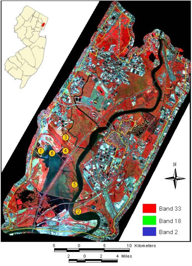
Figure 3. AISA imagery of the New Jersey Meadowlands and the six sites where field spectra were collected (site 1—Harrier Meadow; site 2—The Bend; site 3—The Turn; site 4—Station 8; site 5—Saw Mill Creek; and site 6—The Dock).
Landscape Metrics and Spatial Pattern Analysis
Spatial pattern metrics were calculated from the 40 sampled sites using Fragstats, analysis software that can calculate a wide variety of landscape metrics from a thematic map (McGarigal & Marks, 1995). Metrics calculated in this study were class-level metrics of total class area per hectare (CA), number of patches (NP), total edge in meters (TE), and fractal dimension index (FDI), as well as the landscape-level metrics of patch richness (PR) and the Shannon Diversity Index (SHDI). Descriptions of, and calculation equations for, these metrics are presented in Table 2.
Results
Marsh Surface Classification
Each spectral class in the MNF band image represented a relatively homogenous and distinct plant assemblage or substrate type in the Meadowlands marsh. We scored each class against known surface spectra with the SAM, and each pixel in the thematic map was accordingly assigned to a single marsh surface. We then merged and renamed the classes into the following seven predefined surface area types (Figure 4): Distichlis spicata and Spartina patens were defined as a single High Marsh type, since these two species define the high marsh community in the Meadowlands. The Phragmites type was characterized by tall (> 2 m) dense monotypic stands of Phragmites australis with 100% cover. The Stunted Phragmites type was characterized by a monoculture of low-density Phragmites not exceeding two meters in height and a vegetation-to-mud-cover ratio of 50:50 or greater. The High Marsh/Phragmites type was defined as a mixture of sparse Phragmites stems with an understory of high marsh grasses (Spartina patens and Distichlis spicata). The Spartina type was characterized by dense stands of Spartina alterniflora with 90% or more vegetation cover. Exposed mud surfaces were classified into a single Mud type. These mud surfaces were exposed at low tide and free of vascular vegetation. The Water type included open-surface waters in ponds, channels, and creeks. Though no quantitative accuracy assessment was performed, historical vegetation studies (Sipple, 1972) and visual assessments (using one-foot infrared orthophotos) by ecologists familiar with the Meadowlands confirmed that our seven designations of surface-area type closely matched the actual surfaces of several well-known marsh sites.
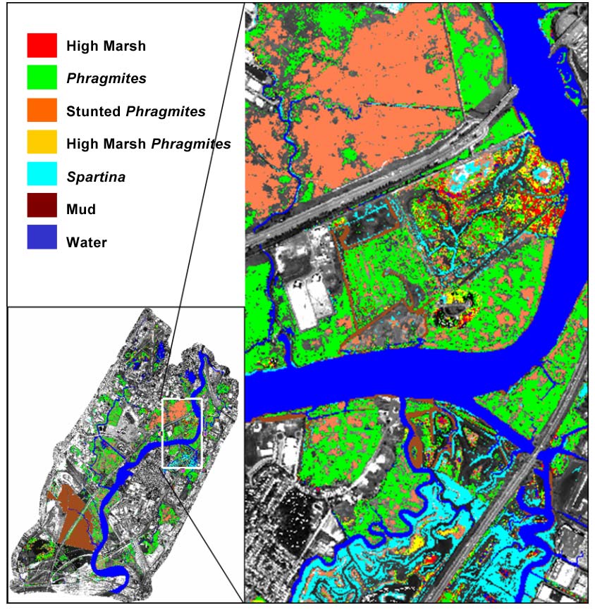
Figure 4. Marsh surface types in the Meadowlands classified using AISA imagery and field-collected spectra.
Class-Level Metrics
We calculated descriptive and test statistics of class-level metrics (CA, NP, TE, and FDI) for five of the seven marsh surface types in tide-open and tide-restricted sites (Table 3). We found that Stunted Phragmites was the most common surface type and existed in both tide-open and tide-restricted sites (N=20 and N=19, respectively). All other surface types were more common in tide-open sites than in tide-restricted sites. Mud was five times more likely to occur in tide-open sites than in tide-restricted sites (N=3 compared with N=15). In terms of class-level metrics, the amount of High Marsh varied most widely between tide-open and tide-restricted sampling sites. High Marsh occupied approximately 13% of the tide-open sites and only 5% of tide-restricted sites. The NP in tide-open sites was almost double that in tide-restricted sites, and consequently the TE was longer at tide-open sites than in tide-restricted sites. The FDI, a measure of patch-shape complexity, was also higher at tide-open sites than at tide-restricted sites (1.11 compared with 1.07; p < 0.05). The CAs of Stunted Phragmites and Water were not significantly different between the two tidal regimes. However, the NP and TE of both Stunted Phragmites and Water were twice as high in tide-open sites. In other words, twice as many patches of these two surface types were found in tide-open sites than in tide-restricted sites, but the total area of these types was no different based on tidal regime. The CA of the Phragmites surface type was similar in both tidal regimes, and so were the NP and the FDI. The only exception was the TE, which was marginally significant (at p < 0.05).
Landscape-Level Metrics
Table 4 presents the descriptive and test statistics calculated for the landscape-level metrics (PR and SHDI) between tide-restricted and tide-open sites. PR is simply the number of different patch types. Overall, tide-open sites had a larger mean number of patch types (4.85) than the tide-restricted sites (3.60). Similarly, tide-open sites had a significantly higher SHDI than tide-restricted sites (1.135 compared with 0.679). This indicates that the distribution of area among patch types was more even in tide-open sites than in tide-restricted sites. The distribution of the SHDI between tide-restricted and tide-open sites was also graphed in a Q-Q plot (Figure 5). All points in the graph were above the y = x line, indicating SHDI in tide-open sites was on average 0.6 larger than that in tide-restricted sites (points would be gathered around the y = x line if the sites showed similar distribution).
Figure 5. Q-Q plot of the Shannon Diversity Index (SHDI) calculated for tide-open and tide-restricted marsh in the Meadowlands. The SHDI is on average 0.6 higher in tide-open marsh than in tide-restricted marsh.
Discussion
Our approach consisted of classifying hyperspectral imagery based on field-collected spectra of the dominant marsh surface types that make up the ecologically significant surfaces and plant communities in the New Jersey Meadowlands. Based on the scale of this study, it was clear that there were significant differences in landscape metrics between tide-restricted and tide-open sites. At the landscape level, tide-open sites had a greater number of patch types, and the distribution of these patches was more even. At the class level, Stunted Phragmites was the most common surface type under both tidal regimes. Another significant feature at the class level was the extent and configuration of the High Marsh type. There was more CA, NP, and TE of this type in tide-open sites than in tide-restricted sites. There were no significant differences in the total area and spatial arrangement of the Phragmites surface type between tide-restricted and tide-open sites. Overall, we found that at the class level, the NP and TE were the best landscape metrics for determining whether marsh surface types are tide-open or tide-restricted.
The results also indicated that it might be possible to determine tide restriction from hyperspectral remote sensing images alone using landscape metrics. The images were able to reveal marsh features such as ponds, pannes, levees, and back marsh stands that are ecologically significant and measurable. This implies that an unsupervised computer-learning algorithm might be developed to calculate landscape metrics from remote sensing images and then automatically classify tide-restricted areas from the images to arrive at an assessment of the overall biodiversity or state of a given ecosystem. Similar methods could be devised to detect and assess habitat availability and biodiversity of riverbank vegetation that has been modified by flooding or by other disturbances, such as fires, landslides, and erosion, that might periodically affect the spatial arrangements of land cover.
In our case, we assumed the minimum mapping unit to be 2.5 by 2.5 meters (image pixel size) and the sample size to be 100 by 100 meters. It was within these resolutions that classes and patches were identified. It is not clear how altering the mapping unit and sample size might affect the identification of spectral classes and surface patches within the hyperspectral imagery. This is important because marsh species diversity has been found to be proportional to the size of the marsh patches (Kane, 1987). It appears safe to assume that sample size ultimately has a direct effect on the overall estimation of habitat heterogeneity (Mayer & Cameron, 2003). Our chosen scale may be appropriate to address the persistence of vascular plant and vertebrate animal species but inadequate for addressing species that operate at larger and smaller scales, such as migrating birds and microinvertebrates.
Instead of using fixed plots in future studies, we suggest selecting sampling sites—especially irregular polygons—from existing patches, as they would be a better reflection of the nature of marsh fragments. Irregular polygons would allow the inclusion of information on marsh edges as additional metrics for identifying and characterizing marsh fragments in the landscape. Further studies are needed to establish a reliable relationship between scale, habitat heterogeneity, and biodiversity.
*Except where noted, measurements throughout this paper are in metric notation; conversions to U.S. equivalents can be obtained at http://www.onlineconversion.com/length.htm.